ゼロから作るDeep Learning実践【2025年AI開発入門】

2025年、AIは誰もが使える技術になりましたが、その仕組みを理解している人は少数です。本記事では、NumPyだけでニューラルネットワークをゼロから実装し、Deep Learningの本質を理解します。

なぜゼロから作るのか

フレームワークの裏側を理解する

理解レベル	できること	できないこと
フレームワーク利用のみ	モデル実装、学習	カスタム層、最適化手法の開発
ゼロから実装経験あり	上記 + 独自アーキテクチャ設計	-

ニューラルネットワークの基礎

パーセプトロン

import numpy as np

def perceptron(x, w, b):
    """
    単純パーセプトロン
    x: 入力（2次元）
    w: 重み
    b: バイアス
    """
    return 1 if np.dot(x, w) + b > 0 else 0

# ANDゲートの実装
def AND(x1, x2):
    w = np.array([0.5, 0.5])
    b = -0.7
    return perceptron(np.array([x1, x2]), w, b)

# テスト
print(AND(0, 0))  # 0
print(AND(0, 1))  # 0
print(AND(1, 0))  # 0
print(AND(1, 1))  # 1

# ORゲートの実装
def OR(x1, x2):
    w = np.array([0.5, 0.5])
    b = -0.3
    return perceptron(np.array([x1, x2]), w, b)

# NANDゲートの実装
def NAND(x1, x2):
    w = np.array([-0.5, -0.5])
    b = 0.7
    return perceptron(np.array([x1, x2]), w, b)

# XORゲート（多層パーセプトロン）
def XOR(x1, x2):
    s1 = NAND(x1, x2)
    s2 = OR(x1, x2)
    return AND(s1, s2)

print(XOR(0, 0))  # 0
print(XOR(0, 1))  # 1
print(XOR(1, 0))  # 1
print(XOR(1, 1))  # 0

活性化関数

import numpy as np
import matplotlib.pyplot as plt

# ステップ関数
def step_function(x):
    return np.where(x > 0, 1, 0)

# シグモイド関数
def sigmoid(x):
    return 1 / (1 + np.exp(-np.clip(x, -500, 500)))

# ReLU関数
def relu(x):
    return np.maximum(0, x)

# Leaky ReLU
def leaky_relu(x, alpha=0.01):
    return np.where(x > 0, x, alpha * x)

# tanh関数
def tanh(x):
    return np.tanh(x)

# Swish関数（2025年推奨）
def swish(x):
    return x * sigmoid(x)

# 可視化
x = np.linspace(-5, 5, 100)
plt.figure(figsize=(12, 8))

plt.subplot(2, 3, 1)
plt.plot(x, step_function(x))
plt.title('Step Function')
plt.grid()

plt.subplot(2, 3, 2)
plt.plot(x, sigmoid(x))
plt.title('Sigmoid')
plt.grid()

plt.subplot(2, 3, 3)
plt.plot(x, relu(x))
plt.title('ReLU')
plt.grid()

plt.subplot(2, 3, 4)
plt.plot(x, leaky_relu(x))
plt.title('Leaky ReLU')
plt.grid()

plt.subplot(2, 3, 5)
plt.plot(x, tanh(x))
plt.title('tanh')
plt.grid()

plt.subplot(2, 3, 6)
plt.plot(x, swish(x))
plt.title('Swish')
plt.grid()

plt.tight_layout()
plt.show()

3層ニューラルネットワークの実装

フォワード伝播

import numpy as np

class ThreeLayerNet:
    def __init__(self, input_size, hidden_size, output_size):
        """
        3層ニューラルネットワーク
        input_size: 入力層のニューロン数
        hidden_size: 隠れ層のニューロン数
        output_size: 出力層のニューロン数
        """
        # 重みの初期化（Heの初期化）
        self.params = {}
        self.params['W1'] = np.random.randn(input_size, hidden_size) * np.sqrt(2.0 / input_size)
        self.params['b1'] = np.zeros(hidden_size)
        self.params['W2'] = np.random.randn(hidden_size, output_size) * np.sqrt(2.0 / hidden_size)
        self.params['b2'] = np.zeros(output_size)

    def predict(self, x):
        """予測（フォワード伝播）"""
        W1, W2 = self.params['W1'], self.params['W2']
        b1, b2 = self.params['b1'], self.params['b2']

        # 第1層
        a1 = np.dot(x, W1) + b1
        z1 = sigmoid(a1)

        # 第2層（出力層）
        a2 = np.dot(z1, W2) + b2
        y = softmax(a2)

        return y

    def loss(self, x, t):
        """損失関数（交差エントロピー誤差）"""
        y = self.predict(x)
        return cross_entropy_error(y, t)

    def accuracy(self, x, t):
        """精度"""
        y = self.predict(x)
        y = np.argmax(y, axis=1)
        t = np.argmax(t, axis=1)

        accuracy = np.sum(y == t) / float(x.shape[0])
        return accuracy

def softmax(x):
    """ソフトマックス関数"""
    if x.ndim == 2:
        x = x - np.max(x, axis=1, keepdims=True)
        return np.exp(x) / np.sum(np.exp(x), axis=1, keepdims=True)
    else:
        x = x - np.max(x)
        return np.exp(x) / np.sum(np.exp(x))

def cross_entropy_error(y, t):
    """交差エントロピー誤差"""
    if y.ndim == 1:
        t = t.reshape(1, t.size)
        y = y.reshape(1, y.size)

    batch_size = y.shape[0]
    return -np.sum(t * np.log(y + 1e-7)) / batch_size

バックプロパゲーション（誤差逆伝播法）

class TwoLayerNet:
    def __init__(self, input_size, hidden_size, output_size):
        # 重みの初期化
        self.params = {}
        self.params['W1'] = np.random.randn(input_size, hidden_size) * 0.01
        self.params['b1'] = np.zeros(hidden_size)
        self.params['W2'] = np.random.randn(hidden_size, output_size) * 0.01
        self.params['b2'] = np.zeros(output_size)

    def predict(self, x):
        W1, W2 = self.params['W1'], self.params['W2']
        b1, b2 = self.params['b1'], self.params['b2']

        a1 = np.dot(x, W1) + b1
        z1 = sigmoid(a1)
        a2 = np.dot(z1, W2) + b2
        y = softmax(a2)

        return y

    def loss(self, x, t):
        y = self.predict(x)
        return cross_entropy_error(y, t)

    def accuracy(self, x, t):
        y = self.predict(x)
        y = np.argmax(y, axis=1)
        t = np.argmax(t, axis=1)

        accuracy = np.sum(y == t) / float(x.shape[0])
        return accuracy

    def numerical_gradient(self, x, t):
        """数値微分による勾配計算（検証用）"""
        loss_W = lambda W: self.loss(x, t)

        grads = {}
        grads['W1'] = numerical_gradient(loss_W, self.params['W1'])
        grads['b1'] = numerical_gradient(loss_W, self.params['b1'])
        grads['W2'] = numerical_gradient(loss_W, self.params['W2'])
        grads['b2'] = numerical_gradient(loss_W, self.params['b2'])

        return grads

    def gradient(self, x, t):
        """誤差逆伝播法による勾配計算"""
        W1, W2 = self.params['W1'], self.params['W2']
        b1, b2 = self.params['b1'], self.params['b2']
        grads = {}

        batch_num = x.shape[0]

        # フォワード
        a1 = np.dot(x, W1) + b1
        z1 = sigmoid(a1)
        a2 = np.dot(z1, W2) + b2
        y = softmax(a2)

        # バックワード
        dy = (y - t) / batch_num
        grads['W2'] = np.dot(z1.T, dy)
        grads['b2'] = np.sum(dy, axis=0)

        dz1 = np.dot(dy, W2.T)
        da1 = sigmoid_grad(a1) * dz1
        grads['W1'] = np.dot(x.T, da1)
        grads['b1'] = np.sum(da1, axis=0)

        return grads

def sigmoid_grad(x):
    """シグモイド関数の微分"""
    return (1.0 - sigmoid(x)) * sigmoid(x)

def numerical_gradient(f, x):
    """数値微分"""
    h = 1e-4
    grad = np.zeros_like(x)

    it = np.nditer(x, flags=['multi_index'], op_flags=['readwrite'])
    while not it.finished:
        idx = it.multi_index
        tmp_val = x[idx]
        x[idx] = tmp_val + h
        fxh1 = f(x)

        x[idx] = tmp_val - h
        fxh2 = f(x)
        grad[idx] = (fxh1 - fxh2) / (2*h)

        x[idx] = tmp_val
        it.iternext()

    return grad

MNIST手書き数字認識

データセット準備

from keras.datasets import mnist
import numpy as np

# データ読み込み
(x_train, t_train), (x_test, t_test) = mnist.load_data()

# 前処理
x_train = x_train.reshape(-1, 784).astype('float32') / 255.0
x_test = x_test.reshape(-1, 784).astype('float32') / 255.0

# One-hotエンコーディング
def to_one_hot(t, num_classes=10):
    return np.eye(num_classes)[t]

t_train = to_one_hot(t_train)
t_test = to_one_hot(t_test)

print(f"訓練データ: {x_train.shape}")
print(f"テストデータ: {x_test.shape}")

学習

# ネットワーク生成
network = TwoLayerNet(input_size=784, hidden_size=50, output_size=10)

# ハイパーパラメータ
iters_num = 10000
train_size = x_train.shape[0]
batch_size = 100
learning_rate = 0.1

train_loss_list = []
train_acc_list = []
test_acc_list = []

# 1エポックあたりの繰り返し数
iter_per_epoch = max(train_size / batch_size, 1)

for i in range(iters_num):
    # ミニバッチの取得
    batch_mask = np.random.choice(train_size, batch_size)
    x_batch = x_train[batch_mask]
    t_batch = t_train[batch_mask]

    # 勾配計算
    grad = network.gradient(x_batch, t_batch)

    # パラメータ更新
    for key in ('W1', 'b1', 'W2', 'b2'):
        network.params[key] -= learning_rate * grad[key]

    # 損失関数の値を記録
    loss = network.loss(x_batch, t_batch)
    train_loss_list.append(loss)

    # 1エポックごとに精度を計算
    if i % iter_per_epoch == 0:
        train_acc = network.accuracy(x_train, t_train)
        test_acc = network.accuracy(x_test, t_test)
        train_acc_list.append(train_acc)
        test_acc_list.append(test_acc)
        print(f"Epoch {int(i / iter_per_epoch)}: train acc={train_acc:.4f}, test acc={test_acc:.4f}")

# 学習曲線の可視化
import matplotlib.pyplot as plt

plt.figure(figsize=(12, 4))

plt.subplot(1, 2, 1)
plt.plot(train_loss_list)
plt.xlabel('Iteration')
plt.ylabel('Loss')
plt.title('Training Loss')

plt.subplot(1, 2, 2)
epochs = np.arange(len(train_acc_list))
plt.plot(epochs, train_acc_list, label='Train')
plt.plot(epochs, test_acc_list, label='Test', linestyle='--')
plt.xlabel('Epoch')
plt.ylabel('Accuracy')
plt.title('Accuracy')
plt.legend()

plt.tight_layout()
plt.show()

最適化手法

SGD（確率的勾配降下法）

class SGD:
    def __init__(self, lr=0.01):
        self.lr = lr

    def update(self, params, grads):
        for key in params.keys():
            params[key] -= self.lr * grads[key]

Momentum

class Momentum:
    def __init__(self, lr=0.01, momentum=0.9):
        self.lr = lr
        self.momentum = momentum
        self.v = None

    def update(self, params, grads):
        if self.v is None:
            self.v = {}
            for key, val in params.items():
                self.v[key] = np.zeros_like(val)

        for key in params.keys():
            self.v[key] = self.momentum * self.v[key] - self.lr * grads[key]
            params[key] += self.v[key]

AdaGrad

class AdaGrad:
    def __init__(self, lr=0.01):
        self.lr = lr
        self.h = None

    def update(self, params, grads):
        if self.h is None:
            self.h = {}
            for key, val in params.items():
                self.h[key] = np.zeros_like(val)

        for key in params.keys():
            self.h[key] += grads[key] * grads[key]
            params[key] -= self.lr * grads[key] / (np.sqrt(self.h[key]) + 1e-7)

Adam（2025年推奨）

class Adam:
    def __init__(self, lr=0.001, beta1=0.9, beta2=0.999):
        self.lr = lr
        self.beta1 = beta1
        self.beta2 = beta2
        self.iter = 0
        self.m = None
        self.v = None

    def update(self, params, grads):
        if self.m is None:
            self.m, self.v = {}, {}
            for key, val in params.items():
                self.m[key] = np.zeros_like(val)
                self.v[key] = np.zeros_like(val)

        self.iter += 1
        lr_t = self.lr * np.sqrt(1.0 - self.beta2**self.iter) / (1.0 - self.beta1**self.iter)

        for key in params.keys():
            self.m[key] += (1 - self.beta1) * (grads[key] - self.m[key])
            self.v[key] += (1 - self.beta2) * (grads[key]**2 - self.v[key])

            params[key] -= lr_t * self.m[key] / (np.sqrt(self.v[key]) + 1e-7)

最適化手法の比較

# 各最適化手法でMNIST学習
optimizers = {
    'SGD': SGD(lr=0.1),
    'Momentum': Momentum(lr=0.01),
    'AdaGrad': AdaGrad(lr=0.01),
    'Adam': Adam(lr=0.001)
}

results = {}

for optimizer_name, optimizer in optimizers.items():
    network = TwoLayerNet(input_size=784, hidden_size=50, output_size=10)
    train_acc_list = []

    for i in range(1000):
        batch_mask = np.random.choice(train_size, batch_size)
        x_batch = x_train[batch_mask]
        t_batch = t_train[batch_mask]

        grad = network.gradient(x_batch, t_batch)
        optimizer.update(network.params, grad)

        if i % 100 == 0:
            train_acc = network.accuracy(x_train, t_train)
            train_acc_list.append(train_acc)

    results[optimizer_name] = train_acc_list

# 結果の可視化
plt.figure(figsize=(10, 6))
for optimizer_name, train_acc_list in results.items():
    plt.plot(train_acc_list, label=optimizer_name)

plt.xlabel('Epochs')
plt.ylabel('Accuracy')
plt.title('Optimizer Comparison')
plt.legend()
plt.grid()
plt.show()

正則化

Weight Decay（L2正則化）

class TwoLayerNetWithRegularization(TwoLayerNet):
    def __init__(self, input_size, hidden_size, output_size, weight_decay_lambda=0.01):
        super().__init__(input_size, hidden_size, output_size)
        self.weight_decay_lambda = weight_decay_lambda

    def loss(self, x, t):
        y = self.predict(x)
        loss = cross_entropy_error(y, t)

        # Weight Decay
        weight_decay = 0
        for param in [self.params['W1'], self.params['W2']]:
            weight_decay += 0.5 * self.weight_decay_lambda * np.sum(param ** 2)

        return loss + weight_decay

    def gradient(self, x, t):
        grads = super().gradient(x, t)

        # Weight Decayの勾配を追加
        grads['W1'] += self.weight_decay_lambda * self.params['W1']
        grads['W2'] += self.weight_decay_lambda * self.params['W2']

        return grads

Dropout

class Dropout:
    def __init__(self, dropout_ratio=0.5):
        self.dropout_ratio = dropout_ratio
        self.mask = None

    def forward(self, x, train_flg=True):
        if train_flg:
            self.mask = np.random.rand(*x.shape) > self.dropout_ratio
            return x * self.mask
        else:
            return x * (1.0 - self.dropout_ratio)

    def backward(self, dout):
        return dout * self.mask

Batch Normalization

class BatchNormalization:
    def __init__(self, gamma, beta, momentum=0.9, running_mean=None, running_var=None):
        self.gamma = gamma
        self.beta = beta
        self.momentum = momentum
        self.input_shape = None

        self.running_mean = running_mean
        self.running_var = running_var

        self.batch_size = None
        self.xc = None
        self.std = None
        self.dgamma = None
        self.dbeta = None

    def forward(self, x, train_flg=True):
        self.input_shape = x.shape
        if x.ndim != 2:
            N, C, H, W = x.shape
            x = x.reshape(N, -1)

        out = self.__forward(x, train_flg)

        return out.reshape(*self.input_shape)

    def __forward(self, x, train_flg):
        if self.running_mean is None:
            N, D = x.shape
            self.running_mean = np.zeros(D)
            self.running_var = np.zeros(D)

        if train_flg:
            mu = x.mean(axis=0)
            xc = x - mu
            var = np.mean(xc**2, axis=0)
            std = np.sqrt(var + 10e-7)
            xn = xc / std

            self.batch_size = x.shape[0]
            self.xc = xc
            self.xn = xn
            self.std = std
            self.running_mean = self.momentum * self.running_mean + (1-self.momentum) * mu
            self.running_var = self.momentum * self.running_var + (1-self.momentum) * var
        else:
            xc = x - self.running_mean
            xn = xc / ((np.sqrt(self.running_var + 10e-7)))

        out = self.gamma * xn + self.beta
        return out

    def backward(self, dout):
        if dout.ndim != 2:
            N, C, H, W = dout.shape
            dout = dout.reshape(N, -1)

        dx = self.__backward(dout)

        dx = dx.reshape(*self.input_shape)
        return dx

    def __backward(self, dout):
        dbeta = dout.sum(axis=0)
        dgamma = np.sum(self.xn * dout, axis=0)
        dxn = self.gamma * dout
        dxc = dxn / self.std
        dstd = -np.sum((dxn * self.xc) / (self.std * self.std), axis=0)
        dvar = 0.5 * dstd / self.std
        dxc += (2.0 / self.batch_size) * self.xc * dvar
        dmu = np.sum(dxc, axis=0)
        dx = dxc - dmu / self.batch_size

        self.dgamma = dgamma
        self.dbeta = dbeta

        return dx

CNN（畳み込みニューラルネットワーク）の基礎

畳み込み層

class Convolution:
    def __init__(self, W, b, stride=1, pad=0):
        self.W = W
        self.b = b
        self.stride = stride
        self.pad = pad

    def forward(self, x):
        FN, C, FH, FW = self.W.shape
        N, C, H, W = x.shape
        out_h = int(1 + (H + 2*self.pad - FH) / self.stride)
        out_w = int(1 + (W + 2*self.pad - FW) / self.stride)

        col = im2col(x, FH, FW, self.stride, self.pad)
        col_W = self.W.reshape(FN, -1).T

        out = np.dot(col, col_W) + self.b
        out = out.reshape(N, out_h, out_w, -1).transpose(0, 3, 1, 2)

        return out

def im2col(input_data, filter_h, filter_w, stride=1, pad=0):
    """画像を2次元配列に変換"""
    N, C, H, W = input_data.shape
    out_h = (H + 2*pad - filter_h)//stride + 1
    out_w = (W + 2*pad - filter_w)//stride + 1

    img = np.pad(input_data, [(0,0), (0,0), (pad, pad), (pad, pad)], 'constant')
    col = np.zeros((N, C, filter_h, filter_w, out_h, out_w))

    for y in range(filter_h):
        y_max = y + stride*out_h
        for x in range(filter_w):
            x_max = x + stride*out_w
            col[:, :, y, x, :, :] = img[:, :, y:y_max:stride, x:x_max:stride]

    col = col.transpose(0, 4, 5, 1, 2, 3).reshape(N*out_h*out_w, -1)
    return col

プーリング層

class Pooling:
    def __init__(self, pool_h, pool_w, stride=1, pad=0):
        self.pool_h = pool_h
        self.pool_w = pool_w
        self.stride = stride
        self.pad = pad

    def forward(self, x):
        N, C, H, W = x.shape
        out_h = int(1 + (H - self.pool_h) / self.stride)
        out_w = int(1 + (W - self.pool_w) / self.stride)

        col = im2col(x, self.pool_h, self.pool_w, self.stride, self.pad)
        col = col.reshape(-1, self.pool_h*self.pool_w)

        out = np.max(col, axis=1)
        out = out.reshape(N, out_h, out_w, C).transpose(0, 3, 1, 2)

        return out

まとめ：Deep Learning実装の本質

学んだこと

1. ニューラルネットワークの基本：パーセプトロン、活性化関数
2. 学習アルゴリズム：誤差逆伝播法、最適化手法
3. 正則化：Weight Decay、Dropout、Batch Normalization
4. CNN：畳み込み層、プーリング層

次のステップ

• PyTorch/TensorFlow実装：実践的な深層学習
• Transformer：最新のアーキテクチャ
• 強化学習：エージェント開発
• 生成AI：GANs、Diffusion Models

ゼロから実装することで、Deep Learningの本質を理解できました。次はフレームワークを使った実践的な開発に進みましょう！

---

画像生成プロンプト集（DALL-E 3 / Midjourney用）

プロンプト1：ニューラルネットワークの構造図

Neural network architecture diagram showing input layer, hidden layers, and output layer with interconnected neurons. Colorful nodes connected by lines representing weights. Educational AI visualization style, blue and orange gradient, clean scientific illustration.

プロンプト2：バックプロパゲーションの概念図

Backpropagation algorithm visualization showing forward pass (green arrows) and backward pass (red arrows) through neural network layers. Gradient flow diagram with mathematical notation. Technical machine learning style, dark background with glowing connections.

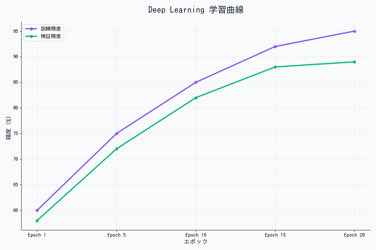
プロンプト3：最適化手法の比較グラフ

Line chart comparing optimization algorithms (SGD, Momentum, AdaGrad, Adam) showing convergence speed. X-axis: epochs, Y-axis: loss/accuracy. Four different colored lines with legend. Professional data visualization style, clean grid, white background.

プロンプト4：CNN畳み込み処理の可視化

Convolutional Neural Network visualization showing image input → convolution filters → feature maps → pooling → output. Step-by-step process diagram with example cat image being processed. Educational deep learning style, colorful layers, modern infographic design.

プロンプト5：MNISTデータセットと予測結果

MNIST handwritten digit recognition visualization. Grid showing original digit images (28x28 pixels) with predicted labels and confidence scores. Correct predictions in green, incorrect in red. Clean machine learning dashboard style, monospace font for numbers.

---

著者について

DX・AI推進コンサルタント
大手企業グループのDX推進責任者・顧問CTO | 長年のIT・DXキャリア | AWS・GA4・生成AI活用を専門に実践ノウハウを発信中

➡️ お問い合わせ・ご相談はこちら

#ディープラーニング #AI #機械学習 #ニューラルネットワーク #Python

---

最終更新: 2025-11-16